Running CFD simulations with OasisMove

Running simulations in OasisMove is performed using a solver based on a incremental pressure correction scheme, as presented in 1. The solver is intended for transient flows in moving domains, and implemented in the NSfracStepMove.py Python file. Problems are solved by running NSfracStepMove, or by using the oasis executable. A problem keyword is required plus any other recognized parameters.

The Moving Vortex problem

To demonstrate how to run problems with OasisMove, we will consider a two-dimensional moving vortex problem inspired by the Taylor-Green vortex problem (see problems/NSfracStep/MovingVortex.py). The problem has an analytical solution of the two-dimensional incompressible Navier–Stokes equations in the absence of body forces, \(\mathbf{f} = 0\), namely

\[\begin{split}\begin{align} \mathbf u(\mathbf x,t) &= (-\sin (2\pi x_2), \sin(2\pi x_1))e^{-4\nu \pi^2 t}\\ p(\mathbf x,t) &= -\cos(2\pi x_1)\cos(2\pi x_2)e^{-8\nu \pi^2 t} \end{align}\end{split}\]

where $mathbf x = (x_1, x_2)$ are the Euclidean coordinates, and \(\nu = 0.025\) \(\text{m}^2\)/s. Furthermore, the mesh velocity \(\mathbf w\) is determined by the following displacement field:

\[\begin{split}\begin{align} \mathbf x(\mathbf \chi,t) &= \mathbf \chi + A \sin \left(\frac{2 \pi t}{T_G}\right) \left(\sin\left(2\pi \frac{\chi_2 + L / 2}{L}\right),\sin\left(2\pi \frac{\chi_1 + L / 2}{L}\right)\right)\\ \mathbf w (\mathbf \chi, t) &= \frac{\partial \mathbf x}{\partial t} \end{align}\end{split}\]

where \(\mathbf \chi = (\chi_1, \chi_2)\) are the ALE coordinates, \(A=0.08\) is the amplitude, \(T_G=4T\) is the period length of the mesh motion, \(T\) is the length of one cycle, and \(L=1\). To simulate this flow problem in OasisMove you can simply type:

oasis NSfracStepMove problem=MovingVortex

or as an alternative:

python NSfracStepMove.py problem=MovingVortex

and the simulation will start. When the simulation is finished, there will be a folder named results_moving_vortex, which contains all simulation results per run. Running the moving vortex problem should produce the following velocity field, here visualized in ParaView over four snapshots from \(T=0.25\) to \(T=1\).

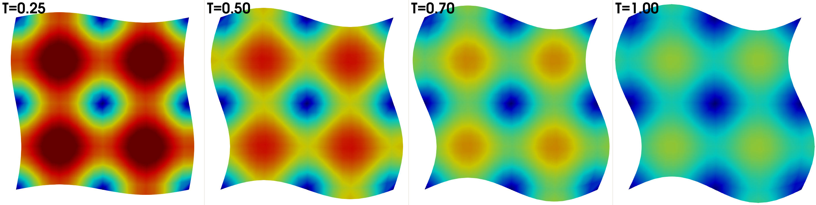
Figure 1: Velocity field over four snapshots for the moving vortex problem on a moving mesh.

Features and issues

The existing software provide many degrees of freedom, however, if you are interested in a specific flow problem not part of OasisMove or want to add additional functionality, please do not hesitate to propose enhancements in the issue tracker, or create a pull request with new features. Similarly, we highly appreciate that you report any bugs or other issues you may experience in the issue tracker.

1

Simo, J.C. and Armero, F. “Unconditional Stability and Long-Term Behavior of Transient Algorithms for the Incompressible Navier-Stokes and Euler Equations”, Computer Methods in Applied Mechanics and Engineering, 1994, (111), 111-154.